The heat equation is an important thing, as I have hopefully conveyed, even in a small part, by posting on Fourier analysis. Most readers would be fairly familiar with the Laplacian  , making its appearance in the heat equation as

Ed Nelson said, “The Laplace operator, or Laplacian, is the most important of all differential operators.” Since I regard Nelson as someone with excellent taste, I think we should pay attention. Indeed, this is such an important concept that it has even made its way into graph theory. When ideas migrate from one field to another; it shows their vitality and depth. Much of the work on the hypergraph Laplacian was in fact inspired by the use of the Laplacian in compact Riemann surfaces, but let’s not get ahead of ourselves… At the same time, concepts should not be migrated to other areas without justification; this might lead to meaninglessly generating results that benefit no one. So we should probably ask ourselves why the Laplacian makes sense in a graph-theoretic context. Fortunately, this turns out to be an easy one. The graph Laplacian has quite an esteemed pedigree, being invented (discovered?) by Gustav Kirchoff (whom we shall soon meet again in another post) in 1847 whilst formulating his circuit laws, which led to an examination of spanning trees. Since then, applications have burgeoned, especially in the modern age where analysis of networks has become vitally important.
Before going on to the links with diffusion, I am going to approach this in the spirit of Kirchoff. He was not interested in spanning trees, as such. Rather, he was trying to simplify computation of current at different points in electric circuits. (A mathematical breakthrough so often comes about in an attempt to make calculation easier.) Whilst I’m not going to retrace his steps exactly, I thought it would be worthwhile to look at the Laplacian in this context.
Kirchoff’s current law states simply that:
The total current flowing into a node equals the total current flowing out of a node.
Let us now take a very simple circuit, consisting of three resistors.
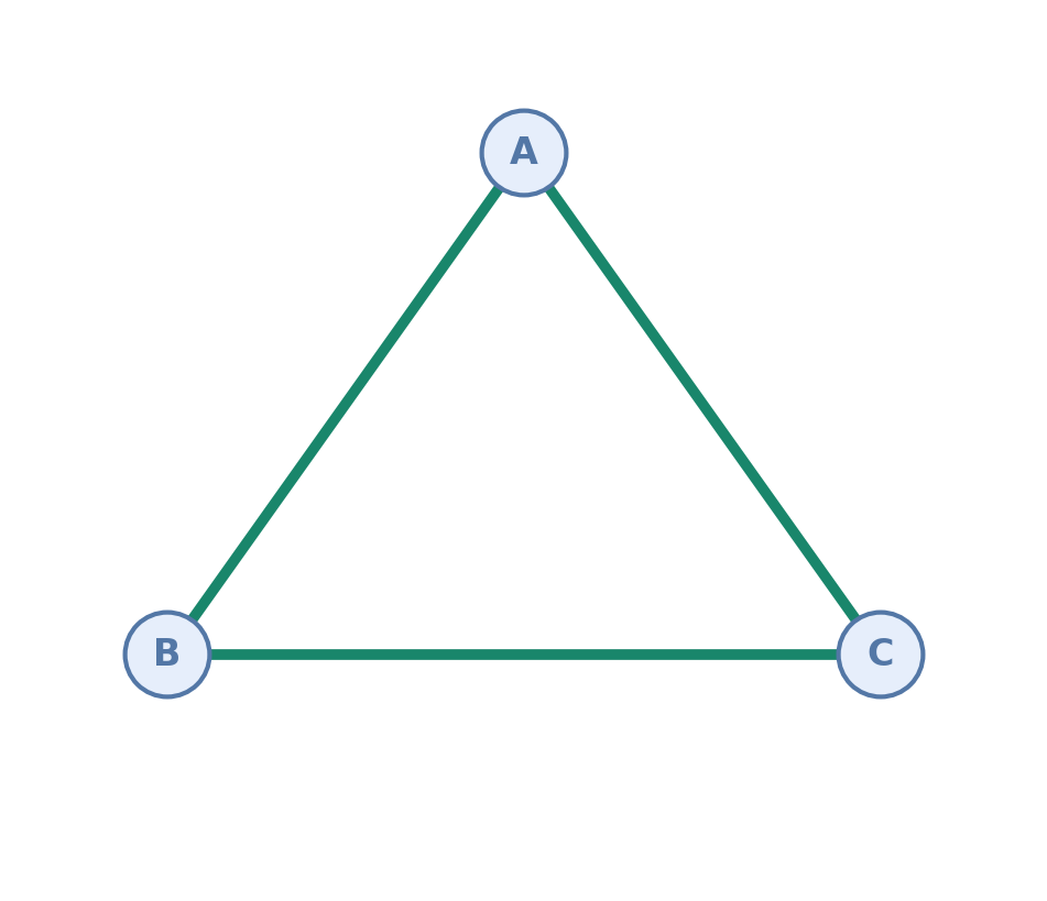
In the above, we imagine that the nodes each have a resistor between them, and we want to determine the current flowing through each node. For now, let’s ignore the power source and assume there is an electrical potential at each of the nodes A, B and C, which we denote  ,
 and
 (we will be working with the potential differences only, so we don’t need to establish a reference for the potential). We assume the resistors between the nodes have resistances
 ,
 and
 , respectively. The (multiplicative) inverse of resistance is conductance, denoted by
 . Applying Ohm’s law
 , we have the system of equations


Applying Kirchoff’s circuit law, we have the following expressions for the current through each node:


(Convince yourself that this makes sense.) We can write this as

Looking at this system, we can start to make a few guesses about what the Laplacian is good for. Obviously, we have ended up with a simple system of linear equations. The first thing to notice is that our matrix has determinant 0. A  matrix with determinant 0 signifies three vectors in that form a parallelepiped with 0 volume, meaning we have actually have a two- or one-dimensional figure. In other words, these linear equations are not independent. Indeed, it is easily seen that row 1 + row 2 = – row 3. What this means for the graph is that forming the system out of a loop introduces redundancy. We could have constructed our system by only using a spanning tree, saving us some computational time.
The matrix/operator  is what we would call a weighted Laplacian. To get the normal graph-theoretic Laplacian, we take all the resistances above to be equal to 1. It is then evident that we can write the Laplacian as

with  the diagonal matrix with the degree of vertex
 at
 and
 is the incidence matrix, with
 if vertices and
 are connected (
 ) and 0 otherwise. Setting all edge weights to be 1 in the above graph, compute the determinant of each matrix obtained by removing the
 th column and row, for
 How does this correspond to the number of spanning trees? What can we say about the number of independent loops in the graph, remembering that adding any edge to a spanning tree creates a loop? Try this with a graph on 4 vertices, and formulate some conjectures. Compute the eigenvalues of . Now do the same thing for a graph with two components, and see if you can come up with more conjectures. If you are very adventurous, try to prove them…
Relevant reading:
Kirby, E.C., Mallion, R.B., Pollak, P. and Skrzyński, P.J., 2016. What Kirchhoff actually did concerning spanning trees in electrical networks and its relationship to modern graph-theoretical work. Croatica Chemica Acta, 89(4), pp.403-417.


