Primality and duality in linear programming

Duality is an extraordinarily important concept in both linear and nonlinear programming. However, the equivalency of the primal and dual problems is not completely obvious, and difficult to give a geometric interpretation to. However, we can get a pretty good idea of how it works by examining the equivalency of the two problems. The following is mostly based on the notes from AA Ahmadi, but I have expanded them a little. Specifically, I show how you can also solve the dual problem from the primal. (I also recommend these notes for a really intuitive explanation of Farkas’ Lemma.)

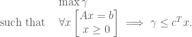
Let us consider the following problem as the primal:

\begin{array}{ll}  & \min  c^T x \\ \text{subject to } &  Ax = b \\ \text{and } &  x\geq 0, \end{array}

where x\geq 0 if each component is \geq 0.

We contend that this problem will have a solution if the dual problem does:

\begin{array}{ll} & \max b^T y \\ \text{subject to } & A^T y \leq c. \end{array}

In both the above problems, we let x,c\in \mathbb{R}^n, b,y \in \mathbb{R}^m and A an m\times n real matrix. When necessary, we shall refer to the primal problem as (P) and the dual as (D). Note that it does not really matter which one you pick as primal or dual, since the dual of the dual has to be the primal again. What we want to do is to show that the primal problem will have a solution as long as the dual one does.

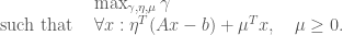
We can start be rephrasing the problem (P) as follows:

\begin{array}{ll}  & \max \gamma    \\ \textrm{ such that } &  \forall x \begin{bmatrix} Ax = b \\ x\geq 0 \end{bmatrix} \implies \gamma \leq c^T x. \end{array}

The strategy here can be seen as maximising the lower bound for c^T x, instead of minimising c^Tx directly. We can rephrase this as an ostensibly stronger problem. The above will have a solution as long as there exist \eta \in \mathbb{R}^m, \mu \in \mathbb{R}^n with \mu \geq 0 such that

\forall x \quad c^T x - \gamma = \eta^T (Ax-b) +\mu^T x.

The stronger problem can now be reformulated as

\begin{array}{ll} & \max_{\gamma, \eta, \mu } \gamma  \\ \text{such that } & \forall x:  \eta^T (Ax-b) +\mu^T x, \quad \mu \geq 0. \end{array}

Now, affine functions of x will be equal everywhere if and only if their coefficients are equal, hence the problem can be written as

\begin{array}{ll} & \max \gamma \\ \textrm{such that } & c = A^T \eta + \mu \\ & \gamma = \eta^T b \\& \mu \geq 0. \end{array}

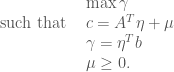
But this is the same as solving the problem

\begin{array}{ll} & \max b^T y \\ \textrm{such that } & A^T y \leq c \\  \end{array}

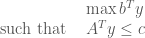
which is the dual problem. Thus, being able to solve the dual problem means we can solve the primal problem. Conversely, suppose that we can solve the primal problem. We phrase the dual problem as

\begin{array}{ll} & \min \gamma \\ \textrm{ such that } & \forall y \quad  A^Ty \leq c \implies b^Ty \leq \gamma \end{array}

The dual problem can be solved if there exists some \mu \geq 0 such that:

\forall y \quad \gamma - b^T y   =  \mu^T (c-A^T y).

This just means that, since \mu is nonnegative, c - A^Ty \geq 0 implies that \mu^T (c-A^T y) is also nonnegative, meaning that we have a nonnegative \gamma - b^T y, and we can minimise \gamma to be as close to b^T y as possible. Once again, we look at the coefficients in the above affine function of y, and can set them to be equal. We therefore get the problem

\begin{array}{ll}  \min  &\gamma = c^Tx  \\ \textrm{such that } &  A x= b\\ & x \geq 0, \end{array}

which is of course just the primal problem again.

The usefulness of primality and duality is not limited to spaces such as \mathbb{R}^n. In fact, these basic concepts will hold for any vector lattice, which allows us to do things like semidefinite programming.