I have taken an interest in regularity lemmas recently, starting with the weak regularity lemma of Frieze and Kannan (in order to understand Szemerédi’s theorem on arithmetic progressions), and decided that I needed to understand the proof of the full regularity lemma. The reference I’m using is Reinhard Diestel‘s book Graph Theory. The regularity lemma seems almost magically powerful to me, and has many applications (and generalisations, but we’ll get to that), but the proof is not all that hard. This post won’t present the full proof, just an overview to get the feel of it. (For another perspective on the regularity lemma by someone who actually knows what he is doing, see Yufei Zhao’s blog entry https://yufeizhao.wordpress.com/2012/09/07/graph-regularity/.)
Much like certain proofs of Roth’s theorem, the idea behind the proof of the regularity lemma is to increase a bounded positive quantity by a constant in each iteration. There are only so many times you can do this, and when you stop, what is left must satisfy the conditions of the lemma. Firstly, some definitions.
Definition 1. Let  be a graph. We say that a pair of disjoint subsets
  is
is  -regular if

for any subsets  and
and  for which
  and
and  .
.
In the above,  as usual denotes edge density

between  and
and  .
.
Definition. Let  be given and let ,
  , be a graph. We say that a partition
  of the vertices of the graph is -regular if


- Each pair
 ,
,  is -regular for all but at most
  of the possible pairs.
The regularity lemma (in one form; there are several equivalent ones) can be stated as follows.
Regularity Lemma. Give some and some  , there exists an integer
  such that any graph
  of order at least
  admits an -regular partition
  where
where  .
.
The quantity that we will bound is a kind of  norm on the graph. If
  and disjoint, set
where  . It should be clear that
  . In effect, we consider
  as a bipartite graph. If the graph is complete,
  will be
  , and
, and  when empty. It does not seem to me that the quantity has a very intuitive meaning. However, it does satisfy the conditions of being bounded and increasing under successive partitions, which is what we’ll need. Suppose that
  is a partition of
  and
and  is a partition of
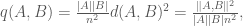
  . We define
 .
.
The fundamental fact which we can prove (quite easily) is that, with all objects as above,

If we have a partition  of the graph
  , we define

We can now prove from the above that if  is a refinement of the partition
  , then

We can already start to spy the strategy of the proof here – we have a bounded quantity that increases with further partitions. What we have to prove is that such refinement of partitions will increase by a fixed amount, which means that it can be done only a bounded number of times, given that is bounded by  .
.
Suppose we are now given a partition of  , namely
  , where all the members except
  have the same size. We regard as a set of members of the partition itself, each a singleton. We set

and define the quantity for our partition  as
as  . With our definitions in place, we can start assembling the required lemmas.
Lemma 0. From the Cauchy-Schwarz inequality, we can conclude that

We won’t be using this lemma in this post (hence calling it Lemma 0), but it is essential in working out the details of the following lemmas.
Lemma 1. If  are disjoint and not
  -regular, there are partitions
  of and
  of such that
For the proof, we pick the sets  and
and  to be two sets of sizes no less than
  and
and  , respectively, witnessing the irregularity of
  , and
, and  and
and  to be what is left over in and .
Using Lemma 1, we can prove the following crucial lemma.
Lemma 2. Let be such that  . If
. If  is an -irregular partition of where
  and , then there is a partition
 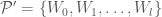 ,
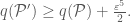
,  , of such that
  and
and 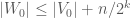 such that
The crucial part here is that the constant increased by does not depend on any of the parameters except . The idea behind the proof of Lemma 2 is to compare all pairs of sets  in the first partition, that might be irregular, then use Lemma 1 to partition them. We take a common refinement of all of these partitions, then partition further to obtain sets of equal cardinality, shunting all the vertices left over into .
What astounds me about Lemma 2 is how wasteful it seems to be. We just partition according to Lemma 1 until we get the desired refinement, and yet this is still powerful enough to lead directly to the result we’re after.
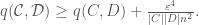
We can now carefully pick our constants and iterate Lemma 2 until we obtain the regularity lemma. Pick such that  . We will need to determine the constants and , depending on but not on . These depend on how many times we have to implement Lemma 2, and how many further partitions each use of Lemma 2 creates. Because the -value of a partition cannot be greater than , we know that the number of iterations has to be bounded by
  . Now, at each stage the cardinality of the exceptional set may increase by
  , if we start with a partition
  . We want to prevent the size of the exceptional set at any stage from exceeding
  , and since we start with some
  with
with  , we have to make sure that
  iterations of adding
  do not exceed
  either. (This is not precise, since the exceptional set will not actually increase by the same factor at each stage, but this will certainly do.) Now
  must be chosen large enough so that for the initial exceptional set , we have a large
  so that
  and . The exceptional set should be allowed up to members, to ensure we have equal cardinality for all the other sets. If
  is large enough to allow
  , we have
  and
and

for  .
.
What is left is to choose . We choose larger than the maximum of  and the number of sets (non-exceptional) that can be generated by applications of the previous lemma, that is, iterations of
  elements of the partition increasing to
  elements.
As long as our graph is relatively small, it is easy to show that a suitable partition exists. If the graph has order , where  , we choose
  and let
  . For
. For  , we want to start with a partition which satisfies
  for Lemma 2 to be valid. Let be as we established above. Now, let
  be a minimal subset of so that divides
  . We then partition into sets of equal cardinality. Because
  , Lemma 2 is applicable, and we simply apply it repeatedly to obtain the partition we are after.
