Dedicated to the memory of Willem L Fouché who, amongst many other stellar contributions to my life, told me to go read Dym & Mckean, and also taught me the connections between Fourier analysis and descriptive set theory.
It’s all well and good to learn advanced mathematics because it’s interesting to you or useful. Not everyone is interested in the history or origin of a field, and that is perfectly fine. For myself, I do not feel I fully understand something until I have some sense of how it originated and more importantly, why. I occasionally discuss Fourier analysis on this blog, because I think it is kind-of magical and because I feel like I don’t have a deep, intuitive understanding of it yet. Recently, I’ve been considering the question whether Fourier analysis was inevitable. Without necessarily going back through the historical record in detail, what would be my guess as to how it came about? This post should perhaps be regarded as historical fiction – an account of how things might have happened.
Since little (but not nothing) happens in a vacuum, let us start with the heat equation, which – as we’ve established – Fourier was obsessed with. Without giving initial or boundary conditions then, we’re looking at the equation

when we’re only considering one dimension.
How do you solve a problem in mathematics? By some combination of two things:
- Solve an easier but related problem, or
- breaking it up into bits you can solve.
We’ll use this combination to try to puzzle out how Fourier analysis could have come about.
The heat equation is not difficult to get a general solution for, if we leave out the initial and boundary conditions. By separating variables and setting 

Since the first two parts depend on different variables, they need to be equal to a constant. Using a minus sign in front of 

Of course, this works for 

Now, a differential equation usually isn’t much use without some initial and boundary conditions, so let’s suppose we’re looking at something (a rod, perhaps) of unit length, whose ends are kept a zero degrees:

To ensure this is satisfied, we can set 


It’s going well so far, but what about the initial conditions? This is where it gets interesting. But making it too interesting makes it very difficult, so let’s start with the easiest possible case. Since the initial condition is given by

we surely can’t get any simpler than setting 


(We only take integer multiples in the argument of 

Great! We’ve solved the problem for a whole class of functions. The question becomes: exactly how big is this class? And can we use this method to expand this class?
Fourier’s audacity was to say that, if we allow 
Fair enough, but this part of the story is still not obvious. Perhaps Fourier had a suspicion that functions can be expanded as sums of trigonometric functions, but how do you go about verifying that? I can only imagine that an enormous amount of work went into this. Nowadays, it is the work of a few minutes to write a script that will output the visualization of a trigonometric sum of the above type. In Fourier’s day, this all had to be done by hand. This might seem like a disadvantage, but I’m not so sure. You would need to think deeply on what you would spend your time on, and choose your problems with care. I’m not against the widespread use of computing in mathematics, but I do think we can learn something from the work habits of the old masters.
So, we can assume that Fourier (like his contemporaries) was an absolute wizard at calculus. If I had to reconstruct his thought process – albeit through a modern lens – I would imagine it went something like the following.
Fourier didn’t have function spaces and orthonormal bases to play around with – even the basic concepts of set theory were still decades away (and Fourier analysis played a crucial role in Cantor’s work, too). But he probably would have been exquisitely aware of the following integral:

and

If we now take the trigonometric series 

Using the identity above, we can conclude that

In other words, if we assume that 
Of course, the mathematical world did not immediately accept Fourier’s methods, with good reason. A lot of work remained to be done. Even today, the convergence of Fourier-type series is an active area of investigation. I can imagine that those who had to use the heat equation in practice welcomed this advance, though. Indeed, it was only a short while before the consequences of this stretched far beyond application to the heat equation…
 ,
, is the permittivity of free space and
  is the magnetic permeability.
 ? Since force is measured in Newton (
 ), we know immediately that Coulomb’s constant has units of
 .
. , which means we can express permittivity in the units
 ? Permittivity is supposed to measure the “polarizability” of a material: a low value means the material polarizes less easily. In order to polarize something, work has to be done, so energy is required, which means part of the potential energy due to two charges is used for the polarization. Therefore, a part of the potential energy is stored in the polarized medium, and the electric field is decreased. A high permittivity leads to a low field intensity, as is evident in a good conductor, which has almost no field inside the substance.
  ,
, 

 represents inductance and

 are easy to compute, we have a quicker way to compute the Fourier coefficients of the convolution, which doesn’t involve computing some ostensibly more difficult integrals. Which requires us to answer the question: why do we want to calculate the convolution in the first place?


 ,
,  ,
,  and
and  . This implies that

 . The contribution of a frequency
  to
to  (in other words, the
 when
when  ,
, , we need to multiply
  and
and  for all values of
  , which leads to our definition.
 the function obtained by integrating

 , we see there is nothing in the above expression that cannot be generalised to any positive real number (we’ll stick to these for now, lest we get lost too early). Supposing
  , we define
 , the above does not work. Instead, we cheat a little by making the lower bound finite:
 used, but we gain the ability to integrate more functions this way. So, we have a fractional integral, but how do we get to the derivative? By remembering the above relation between derivative and integral, we can set
 , which indicates that this is a derivative of order
  -th derivative of a simple function, say
  and the second is the constant 2, the

 is easy enough to compute (use a substitution to turn it into a Gaussian) and is equal to
  . The rest of the integral is not too difficult either – just use the substitution
  . This gives us


 , and suppose the original dice has probability function
  . What if the probabilities are not equal (the die is weighted)?
 and
and  . We can try to make this work by analogy (which is how most mathematics is done). Suppose we have functions
 are random variables over the reals with reader’s choice of appropriate
  -algebra.) We set

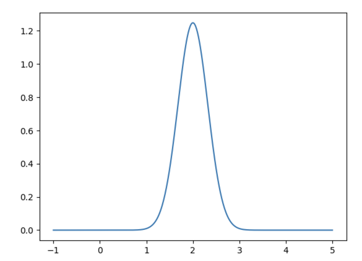
 and
and  , we get the following graphs for the density functions:


 and, by necessity,
  . Letting the hypotenuse be 1, the side adjacent to
  , we have that


 . By replacing
  with
with  , we get

 , we can immediately get Fourier’s identity:

 is some function of distance,
  . We’re not going to discuss how this equation came about and are just going to accept it as it is. There’s a good (but short) post on some of the history
  , in one time variable
  and one space variable
 ![z \in [0,L]](https://s0.wp.com/latex.php?latex=z+%5Cin+%5B0%2CL%5D&bg=ffffff&fg=4c4c4c&s=0&c=20201002) . The given boundary and initial conditions are
. The given boundary and initial conditions are  and
and  . How to formulate these conditions in FEniCS?
  was specified earlier in the code, as usual. In my case, I wanted
 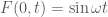 , so I set
 ![g(x[0],t) = (1-x[0])*\sin \omega t](https://s0.wp.com/latex.php?latex=g%28x%5B0%5D%2Ct%29+%3D+%281-x%5B0%5D%29%2A%5Csin+%5Comega+t&bg=ffffff&fg=4c4c4c&s=0&c=20201002) . What about the initial condition
. What about the initial condition  in
in  , it is indeed specified. If we want to add Neumann boundary conditions, we don’t need to do anything more – they are included by default.