This post will again not contain anything very advanced, but try to explain a relatively advanced concept by breaking it down into the ideas that led to its formulation. Once again, the star is that wonderful thing, linear algebra. I have gone from really disliking it upon first encounter (as a naive undergrad), to having immense appreciation for the way in which it can illustrate fundamental mathematical concepts. Here, I will first present some computations that could lead to the formulation of the spectral theorem in the finite dimensional case, and in the next installment I will consider instances of the generalisation. This is similar to how I would approach any new mathematical concept, which is first to reduce it to something I have a decent understanding of, before trying to understand it in any generality.
One version of the spectral theorem can be stated as follows:
Theorem. Suppose  is a compact self-adjoint operator on a Hilbert space
  . Then there is an orthonormal basis of which consists of eigenvectors of , and for which each eigenvalue is real.
Recall that a compact operator is a linear operator such that the image of any bounded subset has compact closure. To get a good idea of the Spectral Theorem, we must first get an idea of what a compact self-adjoint operator would be in a finite dimensional setting. For the moment, let us only consider real matrices. Since the adjoint of a matrix is its conjugate transpose, in this case we consider only symmetric matrices. The question of compactness is trivial in this case. Our Hilbert space will just be  with the usual inner (dot) product. In this case, the spectral theorem states that we should be able to find an orthonormal basis of consisting of eigenvectors of our matrix
  , with corresponding real eigenvalues. Let us consider some simple cases.

Since I don’t feel like working this out by hand, I’ll use some Python:
import numpy as np
A = np.array([[3,2,1],[2,2,3],[1,3,5]])
a = np.linalg.eig(A)
print(a)
This gives us the following output:
(array([ 7.66203005,  2.67899221, -0.34102227]),
 array([[-0.3902192 , -0.83831649,  0.38072882],
        [-0.53490509, -0.13015656, -0.83482681],
        [-0.74940344,  0.52941923,  0.39763018]])
Note that the eigenvectors are given as the columns of the array. Now, it would not be too much to expect that the eigenvectors will give us a basis for  . It would be a stretch to expect these to be orthonormal, however. We can test this out quickly:
b = [np.dot(a[1][i],a[1][j]) for i in range(3) for j in range(3)]
print(b)
(If you look at the code, you’ll see that I actually took the dot product of the rows, not the columns. Why would this have the same result?)
[0.9999999999999998, -5.551115123125783e-17, 2.7755575615628914e-16, -5.551115123125783e-17, 0.9999999999999998, -4.440892098500626e-16, 2.7755575615628914e-16, -4.440892098500626e-16, 1.0000000000000004]
Those values are awfully close to either 0 or 1, and we can suspect that a precise calculation will probably give us those exact answers. But was this just luck, or would it work on any matrix? Let’s generate a random 4 by 4 matrix, which we multiply by its transpose to make it symmetric (where else do we see this product being used to generate Hermitian operators?):
B = np.random.rand(4,4)
BB = np.matmul(B, B.transpose())
bb = np.linalg.eig(BB)
c = [np.dot(bb[1][i],bb[1][j]) for i in range(3) for j in range(3)]
print(c)
[1.0000000000000007, -8.881784197001252e-16, 5.689893001203927e-16, -8.881784197001252e-16, 1.000000000000001, 1.6653345369377348e-16, 5.689893001203927e-16, 1.6653345369377348e-16, 0.9999999999999989]
Once again, we get entries that are practically 0 or 1, and it seems as if NumPy actually gives us the vectors in the desired form. You can get exact results using symbolic computation, for instance using SymPy:
import sympy as sym
A = sym.Matrix([[3,2,1],[2,2,3],[1,3,5]])
A.eigenvects()
This takes surprisingly long however, and doesn’t tell us much we don’t know. We can now formulate a possible finite dimensional version of the spectral theorem:
Conjecture 1. The eigenvectors of a symmetric  real matrix form an orthonormal basis of .
Let us first check this in the case where the matrix has full rank, and we have  linearly independent eigenvectors. Suppose that
  are linearly independent eigenvectors of with eigenvalues
  . For
. For  :
:

and

Since the dot product is commutative, we must have either that  or
or  . The latter part is clearly what we desire, but what if ? If we take a look at the wording of the Spectral Theorem, we can see that it does not state that any set of eigenvectors form a basis, but that there is a basis which consists of eigenvectors. So if we have, say, that
  and
and  , we can form a new vector
  as follows:
This new vector is also an eigenvector with eigenvalue  :
:

Furthermore, will be orthogonal to  . To get orthonormality, we just normalise . (If there are more than two vectors with the same eigenvalue, we just continue applying the Gram-Schmidt process.) We have therefore used the eigenvectors and
  with the same eigenvalue to find two orthonormal vectors ( and
  ) with the same eigenvalue as before.
We can see that we must now replace Conjecture 1 with one that is more in line with the statement of the Spectral Theorem:
Conjecture 2. Given a real  symmetric matrix , there is a basis of consisting of eigenvectors of .
Now, where could this conjecture go wrong? In the above examples, we had nice, non-zero eigenvalues. So let us consider a matrix in which the columns are linearly dependent, and which has an eigenvalue of 0 with multiplicity 2:

A = np.array([[1,1,1],[1,1,1],[1,1,1]])
np.linalg.eig(A)

(array([-2.22044605e-16,  3.00000000e+00,  0.00000000e+00]),
 array([[-0.81649658,  0.57735027,  0.        ],
        [ 0.40824829,  0.57735027, -0.70710678],
        [ 0.40824829,  0.57735027,  0.70710678]]))
As expected, we only have one non-zero eigenvalue, but we still have three orthonormal eigenvectors. NumPy has kindle normalised them for us, but it is easy to see that our eigenvectors will be multiples of  ,
,  and
and  . Clearly, these are orthogonal, and once again we have an orthonormal basis. (Think of a geometric reason why this case is actually simpler than the case of 3 distinct non-zero eigenvalues.)
All of this seems to support our conjecture (but is, of course, not yet a proof). Perhaps our conjecture can be made more general? Will it not perhaps hold for arbitrary matrices? Let’s pick an arbitrary integer matrix, generated for me by Python, and get its eigenvalues and eigenvectors:
[[ 1467.   418. -1015.]
 [  418.  1590. -1565.]
 [-1015. -1565. -1560.]]

D = np.linalg.eig(C)
print(D)

(array([-2369.06809548,  1115.59533457,  2750.47276091]), array([[ 0.20557476, -0.80791041,  0.55228596],
       [ 0.34091587,  0.58811029,  0.73341847],
       [ 0.91734148, -0.03751073, -0.39633011]]))
We check to see if we have an orthonormal basis:
E = [np.dot(D[1][i],D[1][j]) for i in range(3) for j in range(3)]
print(E)

[1.0000000000000002, 5.551115123125783e-17, 0.0, 5.551115123125783e-17, 0.9999999999999998, -2.220446049250313e-16, 0.0, -2.220446049250313e-16, 1.0000000000000002]
Within computational error, this is definitely what we want. One can have some more fun with this by generating a  matrix and solving for the eigenvectors, but for now, the conjecture looks pretty solid, and we can try to prove it properly (but not here). It is also valuable at this point to look at what the spectral theorem means for the diagonalisability of the matrix.
This has been fairly simple, but the goal is to study the spectral theorem in its full form. I an upcoming post, I will consider some more interesting operators on infinite dimensional spaces.


implies
.
and
, then
.


 be a finite set and
  a positive integer. Define
  to be the set of all
  .
.  in the above definition. One could picture an
  exists if and only if there is an edge (in the usual sense of a graph) between
  and
and  for
for  , plus an edge between
  and
and  .
.![R\subset [N]^2](https://s0.wp.com/latex.php?latex=R%5Csubset+%5BN%5D%5E2&bg=ffffff&fg=4c4c4c&s=0&c=20201002) . For
. For  there exists an
  such that if
  and
and  , then there exist
  ,
,  ,
,  for some integer
  .
. ![R\subseteq [N]^2](https://s0.wp.com/latex.php?latex=R%5Csubseteq+%5BN%5D%5E2&bg=ffffff&fg=4c4c4c&s=0&c=20201002) by letting
by letting  if
if  , where we assume
 ![[N]](https://s0.wp.com/latex.php?latex=%5BN%5D&bg=ffffff&fg=4c4c4c&s=0&c=20201002) is large enough so that
is large enough so that  in
in ![[N]^2](https://s0.wp.com/latex.php?latex=%5BN%5D%5E2&bg=ffffff&fg=4c4c4c&s=0&c=20201002) as a grid. In the latter case, the “lower left” (under the diagonal) part of the grid contains all possible differences a subset of
as a grid. In the latter case, the “lower left” (under the diagonal) part of the grid contains all possible differences a subset of  times, 2 occurs
  times, and so on. Clearly then, if we want to minimise the elements of
  (approximately), which means we have
  occurrences of
  be finite non-empty sets of vertices, and let
  be a tripartite graph on these sets of vertices, thus
  for
for  . Suppose that the number of triangles in this graph does not exceed
  for some
  . Then there exists a graph
  which contains no triangle whatsoever, and such that
  for
for  .
. denotes a quantity that is bounded in magnitude by
  , where
  as
as  . The following discussion is similar to that in
 ![\{1,2,\dots ,n\}=[n]](https://s0.wp.com/latex.php?latex=%5C%7B1%2C2%2C%5Cdots+%2Cn%5C%7D%3D%5Bn%5D&bg=ffffff&fg=4c4c4c&s=0&c=20201002) so that
so that  . Suppose we have three elements of
  are all in
  such that

 , each of cardinality
  , with the vertices of each labelled as
  . The important thing about these sets is that the difference (as follows) will let us recover all elements of
  and
and  if
if  ,
,  and
and  , and
, and  and
and  . (Check that this representation captures all three APs, and no more.)
![A_n = A\cap [1,n]](https://s0.wp.com/latex.php?latex=A_n+%3D++A%5Ccap+%5B1%2Cn%5D&bg=ffffff&fg=4c4c4c&s=0&c=20201002) for some
for some  . Also assume that
  contains no non-trivial arithmetic progressions. What does this mean for the tripartite graph? Especially, how many triangles does our graph contain? Since there are no non-trivial arithmetic progressions, we must have
  .
. to satisfy the above equations and obtain a triangle. How many ways are there to do this? Given some
  , we can pick
  ,
,  and
and  . We therefore look at all triples of the form
  for
for ![m\in [3n]](https://s0.wp.com/latex.php?latex=m%5Cin+%5B3n%5D&bg=ffffff&fg=4c4c4c&s=0&c=20201002) . Given that
. Given that ![A\subseteq [n]](https://s0.wp.com/latex.php?latex=A%5Csubseteq+%5Bn%5D&bg=ffffff&fg=4c4c4c&s=0&c=20201002) , we should get at least
, we should get at least  triangles. But how do we apply the triangle removal lemma here? The form it is in does not immediately lend itself to our problem. Let us rephrase it as follows.
 such that if removing
  edges does not make the graph triangle-free, then the graph must have more than
  triangles.
 edges will not make the graph triangle-free, where
  is slightly smaller than
  . We must then have some
  such that the graph contains at least
  triangles. This is impossible however, since it is easily shown that the upper bound on the number of triangles is also
  . For
. For  , we form
  ,
,  This will gives us an approximation to the eigenvector belonging to the dominant eigenvalue. To get the eigenvalue corresponding to the vector, we observe that the eigenvalue

 if each component is
  .
. 
 ,
,  and
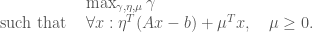
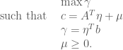
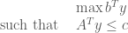
and  real matrix. When necessary, we shall refer to the primal problem as (P) and the dual as (D). Note that it does not really matter which one you pick as primal or dual, since the dual of the dual has to be the primal again. What we want to do is to show that the primal problem will have a solution as long as the dual one does.
 , instead of minimising
  directly. We can rephrase this as an ostensibly stronger problem. The above will have a solution as long as there exist
  ,
,  with
with  such that


 is nonnegative,
  implies that
  is also nonnegative, meaning that we have a nonnegative
  , and we can minimise
  to be as close to
  as possible. Once again, we look at the coefficients in the above affine function of
 . In fact, these basic concepts will hold for any
  and
and  (supposing that these vectors are not parallel). To get a normal vector, we have to get a vector which is perpendicular to both of these. Fortunately, we can assume that we already know about the dot product, and can use it to test for perpendicularity. If there is a vector
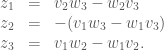
  perpendicular to both of the above, it will have to satisfy the equations
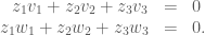
 , and solve for the other two. We therefore get the equations
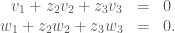

 :
:

 to
to  .)
.) , though. Supposing once again that we are trying to calculate the flow through some surface by approximating the surface with small parallelograms. To find the flow through the surface then, we have to find the part of the flow perpendicular to the parallelogram and multiply with the area. As if by magic though, we already have the surface area of the parallelogram! Specifically, it is given by the magnitude of the normal vector
  and
and  , the area is given by
  (show this!) . This looks familiar, at least, and conforms to the determinant method we usually use to get the area.
  and
and  , since I’m tired of using subscripts. Taking
  as the base, we have the first term,
 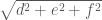 . To get the height, we first take the length of
  projected onto
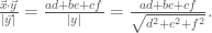
 , we get
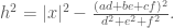

 . What I am interested in is taking a bunch of given matrices (with numerical values) and constants, performing some operations with an unknown matrix, and setting each entry of the final matrix equal to zero and solving. In other words, suppose we are given
  , which are determined beforehand. There is some constant
  which can be varied (this forms part of an iterative scheme), and an unknown matrix
  , which is represented purely symbolically, as such:
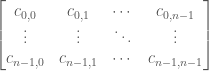
 , and we want to find the entries of
 indicates the
  and
and  to be two arbitrary
  matrices and wanted, for instance, to multiply them, I would use
 for addition.
 be a graph. We say that a pair of disjoint subsets
  is
is  -regular if
 and
and  for which
  and
and  .
. as usual denotes edge density
 and
and  .
. be given and let
  , be a graph. We say that a partition
  of the vertices of the graph is

 ,
,  is
is  of the possible pairs.
 , there exists an integer
  such that any graph
  of order at least
  admits an
  where
where  .
. norm on the graph. If
  and disjoint, set
 . It should be clear that
  . In effect, we consider
  as a bipartite graph. If the graph is complete,
  will be
  , and
, and  when empty. It does not seem to me that the quantity has a very intuitive meaning. However, it does satisfy the conditions of being bounded and increasing under successive partitions, which is what we’ll need. Suppose that
  is a partition of
  is a partition of
  .
.
 of the graph
  , we define
 is a refinement of the partition
  , then
 , namely
  , where all the members except
  have the same size. We regard
 as
as  . With our definitions in place, we can start assembling the required lemmas.
 are disjoint and not
  -regular, there are partitions
  of
of  of
of 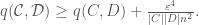
 and
and  to be two sets of sizes no less than
  and
and  , respectively, witnessing the irregularity of
  , and
, and  and
and  to be what is left over in
  . If
. If  is an
is an  and
and  ,
,  , of
, of  and
and  such that
 in the first partition, that might be irregular, then use Lemma 1 to partition them. We take a common refinement of all of these partitions, then partition further to obtain sets of equal cardinality, shunting all the vertices left over into
  . We will need to determine the constants
  . Now, at each stage the cardinality of the exceptional set may increase by
  , if we start with a partition
  . We want to prevent the size of the exceptional set at any stage from exceeding
  , and since we start with some
  with
with  , we have to make sure that
  iterations of adding
  do not exceed
  either. (This is not precise, since the exceptional set will not actually increase by the same factor at each stage, but this will certainly do.) Now
  so that
  and
and  is large enough to allow
  , we have
  and
and 
 .
.  and the number of sets (non-exceptional) that can be generated by
  elements.
  , we choose
  and let
  . For
. For  , we want to start with a partition which satisfies
  for Lemma 2 to be valid. Let
  be a minimal subset of
  . We then partition
  , Lemma 2 is applicable, and we simply apply it repeatedly to obtain the partition we are after.
 , with the usual inner product
 real matrix can be seen as a bounded linear operator
  . (Exercise: Show this.) Since the way in which we “measure” elements of the Hilbert space is through the inner product (and the norm deriving from it), interesting operators would be ones which have some quantifiable relationship with this. For instance, a subspace could be seen as the set of vectors that all satisfy some angular/directional relationship (such as being contained in a plane), and the projection onto this subspace isolates the parts of a vector that satisfy this relationship. So it would seem that a fairly natural question to ask is, which operators will preserve the length and angular relationships between vectors?
 is an operator that takes a vector
  in the same direction as
 . It is easily seen that unless
  , this operator does not preserve inner products, that is,
  . The same goes for translation, that is, an operator that translates any
  to
to  .
. , we see that
 .
. . (This property will be satisfied by all matrices with determinant -1 or 1).
 be the orthogonal projection onto the subspace
  . Then, for any
  ,
, .
. , which is not much different from considering rotations in three dimensions. We immediately run into a problem. If
  ,
, 
 ), it is not too hard to prove, and in the case of irrational ones it would seem sensible from the
![[1,0]](https://s0.wp.com/latex.php?latex=%5B1%2C0%5D&bg=ffffff&fg=4c4c4c&s=0&c=20201002) to the unit vector
to the unit vector ![[0,1]](https://s0.wp.com/latex.php?latex=%5B0%2C1%5D&bg=ffffff&fg=4c4c4c&s=0&c=20201002) , and vice versa. Furthermore, the conjugate transpose of
, and vice versa. Furthermore, the conjugate transpose of  . Thus
  is unitary. Can all of these permutations be seen as rotations?) In fact, any permutation of an orthonormal basis in a Hilbert space is unitary (think of how a permutation of the basis would affect the inner product). Thus, if we think of the shift operator as a permutation of a countable basis, we see that it fits into the general intuition of a unitary operator.
 or
or  ? What does unitary equivalence mean? What does it mean when a unitary operator is self-adjoint? Posing questions like these is, I believe, more valuable than reading a single textbook’s introduction on the subject, because you’re trying to make sense of something in terms of what you already know, and you can allow curiosity to lead you. At some point, the concepts will take on a life of their own and your frame of reference will expand, ready to begin making sense of the next, more advanced concept.