The importance of units and constants

Because I was young and stupid, I never used to pay much attention to constants in physics in my studies. They were just something you had to remember in order to do the calculations, or at least have stored in your calculator. And screw the units – you just needed the number.

Oh, what a sweet summer child I was. Constants and units are the building blocks of understanding physics. Much of physics is about understanding the relationships between various constants, and any new result that provides a link between previously unrelated constants is a major breakthrough. Considering units by themselves may lead to a major breakthrough, as Bohr showed in realizing that Planck’s constant had the units of angular momentum – it is as if nature was inviting us to figure out the principles of quantum mechanics. As for the relationships between constants, one of the most magical formulas of physics to me is the following consequence of Maxwell’s equations:

c^2 = \frac{1}{\varepsilon_0 \mu_0},

where \varepsilon_0 is the permittivity of free space and \mu_0 is the magnetic permeability.

My aim here is not to come up with some amazing conclusion or derivation, but to show that contemplating constants and units might actually lead to a better understanding of the physics, or at the very least serve as a mnemonic aid.

Speaking of electromagnetism, let’s start with that as an exploration of units and constants. We use Coulomb’s law (non-vector form) for the magnitude of the force between two charges as our jumping off point:

F = C\frac{q_1 q_2}{r^2}.

(I’m not going to explain every part of every equation; Wikipedia has all the details.) What does this allow us to say about the Coulomb’s constant, C? Since force is measured in Newton (N), charge in Coulomb (C) and distance in metres (m), we know immediately that Coulomb’s constant has units of

\frac{Nm^2}{C^2}.

Now, we also know from Maxwell that C = 1/4\pi \varepsilon_0, which means we can express permittivity in the units

\frac{C^2}{Nm^2}.

(The danger of removing units rears its ugly head here. Permittivity of a specific material is usually given as a relative permittivity, which is the ratio of the actual permittivity to that of vacuum. This is useful, but does not aid understanding.) Does this tell us anything about \varepsilon? Permittivity is supposed to measure the “polarizability” of a material: a low value means the material polarizes less easily. In order to polarize something, work has to be done, so energy is required, which means part of the potential energy due to two charges is used for the polarization. Therefore, a part of the potential energy is stored in the polarized medium, and the electric field is decreased. A high permittivity leads to a low field intensity, as is evident in a good conductor, which has almost no field inside the substance.

To create a picture of this, consider the atoms comprising our substance. Each atom consists of a positive nucleus surrounded by electrons in their orbital states. Applying an electric field will act “separately” on the protons and the electrons, by the principle of superposition, moving them apart and creating dipoles. This will partially cancel the field, and snap back when the field is removed. The discerning reader might now raise the following question: since vacuum has a non-zero value, does that mean it can be polarized, and energy stored in it? Well, yes – although it is not so easily explained with polarized molecules or atoms. However, there are substances that have even lower permittivities than the vacuum. In addition, the fact that the vacuum can do this is implied by the above relation between c, \mu_0 and \varepsilon_0. Thus, Maxwell’s equations plus the speed of light being finite must imply that there can be energy in free space, without matter to store it. One can appreciate the difficulty of this concept, and the tendency to want to describe this ability to some “aether”, as was common until the end of the nineteenth century.

But back to units. Does understanding the units help us in comprehending the meaning of \varepsilon, which is material-specific? We can simplify the units of \varepsilon slightly by remembering that force times distance is energy, and can write the units as

\frac{C^2}{Jm}

and interpret it as saying “charge squared per Joule per metre”. Since the permittivity of a substance is constant (not really – it depends on frequency), we can perhaps see it as the constant ratio between the product of charges (source of the electric field) and the energy stored through polarization, per metre. How does this help us understand anything? By considering the units of a ubiquitous constant, we have arrived at the doorstep of one of the great breakthroughs of nineteenth century physics, Maxwell’s displacement current. This was a deep insight, especially at a time when science did not have modern atomic concepts.

This isn’t rigorous, and might even be slightly incorrect. But it opens the door to thinking about the physical concepts involved, and leads to deeper insights. In other words, don’t neglect the constants, and don’t think units are superfluous!

Edit: Here’s something else to think about, which may lead to further insight. When you study propagation in cables using the telegrapher’s equations, you will find that the speed of propagation is given by

\frac{1}{\sqrt{LC}}.

Here, L represents inductance and C represents capacitance (look at the units for these as well – I’m glossing over some stuff here). Now, look again at the speed of light in terms of the permittivity and permeability of free space. This gives us a direct analogy: \varepsilon_0 can be seen as the capacitance and \mu_0 as the inductance of free space. At the very least, this is a useful mnemonic device.

Addendum: For another nice discussion on fundamental constants, see Sabine Hossenfelder’s video below.

Fourier analysis – the real story II

One thing I didn’t know about Fourier was his obsession with heat – and not just in the mathematical sense. He literally thought that heat was some sort of panacea. So much so that it contributed to his death! See https://engines.egr.uh.edu/episode/186, for instance.

So, we have the heat equation. How do we solve it? More importantly, how did Fourier solve it? This is somewhat difficult to ascertain, in the general form, for Fourier’s book is written in a manner different from what is today accepted as a mathematical text. First of all, there are many more words and lengthy physical explanations – Fourier’s aim, after all, was not to promulgate a mathematical theory, but a real and useful way of solving the problem of heat in many bodies under many conditions. Of course, we also cannot expect a book from the early 19th century to adhere to our standards of mathematical rigour.

Fortunately, I have come across a great book which starts off with Fourier’s approach to the heat equation, namely “Hot molecules, cold electrons” by Paul J Nahin. If you haven’t read any of Nahin’s books, do yourself a favour. He’s an electrical engineer with a keen appreciation for mathematics, and he makes it a lot of fun. Over the next few posts then, since we’re exploring the origins of Fourier analysis, I thought I would present an argument by Fourier that is recounted in Nahin’s book. I’m not going to go into too much detail, because working that out is part of the fun.

What Fourier was so very good at was solving problems by representing functions as infinite series. It does not seem at first that this would make things simpler, but it does – a lot. Many (including Laplace and Lagrange) were skeptical of Fourier’s methods, and honestly, the techniques did not exist yet to fully justify the methods. Nevertheless, Fourier knew they worked, and he became a titan of mathematics because of them. Here, we will look at his proof for the identity

\frac{\pi}{4} = \cos x - \frac{1}{3} \cos 3x + \frac{1}{5} \cos 5x - \frac{1}{7} \cos 7x + \cdots.

Of course, the first striking thing about this identity is that the right side depends on x
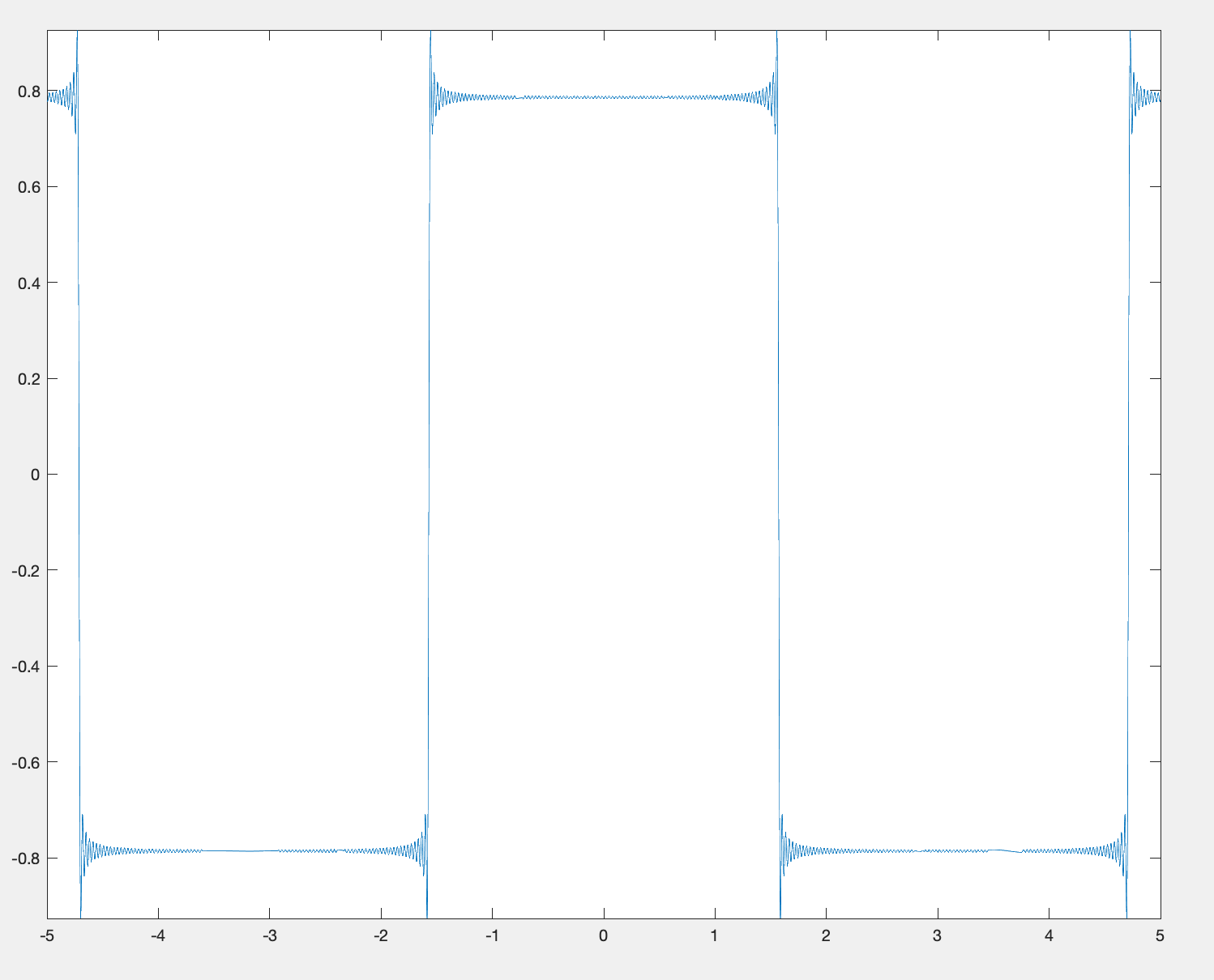
, whilst the left does not. This immediately raises suspicion – as it should, since the identity is not actually correct. Before delving into the derivation, let us approximate the right hand side with some software to see how wrong the identity is. We can use the following in Matlab:

test = @piover4
figure
fplot(test,[-5 5])

function f = piover4(x)
f = 0
for i = 1:100
f = f + ((-1).^(i+1))*cos((2*i -1)*x)/(2*i-1);
end
end

Clearly, the equation is not exactly correct, but it definitely works over a large range of x. By the way, if we want to do this in Python we can use

import numpy as np
import matplotlib.pyplot as plt
def piover4(x):
    sum = 0
    for i in range(1,101):
    sum += (-1)*(i+1)np.cos((2i-1)x)/(2*i-1)
    return sum
xx = np.linspace(-5,5,1000)
yy = piover4(xx)
plt.plot(xx,yy)

The two different values the series converges to over most of the x are probably not too concerning – those are just sign reversals in the series, and we’ll probably see what’s going on there during the derivation. What is much more interesting are the errors near the discontinuities. For the moment, we will park that discussion, although it turns out to be very important. In the next post, we will look at Fourier’s derivation of the identity, and figure out why it’s wrong, but also kind of correct.