convolution | Trying to be a mathematician

Previously, we managed to get an idea of the justification of using convolution by using probabilities, and it seems to make some kind of intuitive sense. But do the same concepts translate to Fourier analysis?

With the convolution product defined as

$(f \star g)(x) = \int f(y) g(x-y) dy,$

(where we leave the limits of integration up to the specific implementation), the key property of the convolution product we will consider is the following:

$\widehat{ (f \star g)}(n) = \hat{f} (n) \hat{g} (n).$

One possibility that immediately presents itself is that, if the Fourier coefficients of $f$ and $g$ are easy to compute, we have a quicker way to compute the Fourier coefficients of the convolution, which doesn’t involve computing some ostensibly more difficult integrals. Which requires us to answer the question: why do we want to calculate the convolution in the first place?

Let’s take some easy functions and see what happens when we take the convolution. Let

$f (t) = \sin 2\pi t \textrm{ and } g (t) = \cos 2\pi t.$

The Fourier coefficient of these functions are really easy to compute, since we have

$\sin 2\pi t = \frac{e^{2\pi i t} - e^{-2\pi i t}}{2i}$

and

$\cos 2\pi t = \frac{e^{2\pi i t} + e^{-2\pi i t}}{2},$

meaning that $\hat{f}(1) = 1/2i$ , $\hat{f} (-1) = -1/2i$ , $\hat{g} (1) = 1/2$ and $\hat{g} (-1) = 1/2$ . This implies that

$\widehat{(f \star g)} (-1) = -\frac{1}{4i}, \widehat{(f \star g)}(1) = \frac{1}{4i}.$

This allows us to immediately write down the convolution product:

$(f \star g)(t) = \frac{1}{4i} \left( e^{2\pi i t} - e^{-2\pi i t} \right) = \frac{1}{2} \sin 2\pi t.$

Clearly, our two signals modify each other. How is this significant? The best way to think of this is as an operation taking place in the frequency domain. Suppose $f$ is our “original” signal, and it is being “modified” by $g$ , yielding a signal $h = f \star g$ . The contribution of a frequency $n$ to $h$ (in other words, the $n$ -th Fourier coefficient), is the $n$ -th Fourier coefficient of $f$ multiplied by the $n$ -th coefficient of $g$ . We can see this as a way of affecting different frequencies in a specific way; something we often refer to as filtering.

We often think of the function in the time domain as the primary object, but looking at the Fourier coefficients is, in a way, far more natural when the function is considered as a signal. Your hear by activating certain hairs in the inner ear, which respond to specific frequencies. In order to generate a specific sound, a loudspeaker has to combine certain frequencies. To modify a signal then, it is therefore by far the easiest to work directly on the level of frequency. Instead of trying to justify the usual definition of convolution, we see the multiplication of Fourier coefficients as the starting point, and then try to see what must be done to the “original” functions to make this possible. So, we suppose that we have made a new function $h$ that has Fourier coefficients formed by the product of the Fourier coefficients of $f$ and $g$ , and try to find an expression for $h$ :

$h(x) = \int \hat{f} (\xi ) \hat{g} (\xi ) e^{2\pi i \xi x} d\xi.$

If you simply write out the definitions in the above, and you remember that

$\int e^{2\pi i y (\xi - \zeta)} dy = 0$ when $\xi \neq \zeta$ ,

you will get the expression for the convolution product of $f$ and $g$ . As such, the definition of convolution has to be seen as a consequence of what we would like to do to the signal, rather than the starting point.

We still have not related the definition to how convolution originated in probability, as detailed in the previous post. Unfortunately, the comparison between the two cases is not exact, because in the probabilistic case we obtain a completely new measure space after the convolution, whereas in the present case we require our objects to live in the same function space. Again, the solution is to think in frequency space: to find all ways of getting $e^{-2\pi i x \xi}$ , we need to multiply $e^{-2\pi (x-y)\xi}$ and $e^{-2\pi i y \xi}$ for all values of $y$ , which leads to our definition.

(As always, I have been rather lax with certain vitally important technicalities – such as the spaces we’re working in and the measures – such as whether we’re working with a sum or an integral. I leave this for the curious reader to sort out.)

You can’t even begin to do Fourier analysis without knowing about the convolution product. But this is a difficult thing to grasp intuitively. I know that I spent many hours trying to understand what’s really going on. There are, as always, really good videos on YouTube about this, which probably explain it better than I ever could, and I urge you to check them out. As for me, when I want to understand something I have to ask why this thing originated, and what it was initially used for. Something like the convolution product does not just drop out of the sky – it had to have some very definite and concrete purpose.

Fortunately, there’s a nice entry at https://math.stackexchange.com/questions/1348361/history-of-convolution that pointed me in the right way – specifically to Laplace, and the theory of probability. Let’s say you have two dice, with sides numbered from 1 to 6 as usual. What is the probability of rolling a seven? To count this we take, say, 1 and asked what should be added to make 7, which is of course 6. We do this for every other number from 2 to 6 (not taking symmetry in to account), and we add the products of the individual probabilities. In other words,

$p(1)p(6)+p(2)p(5)+\cdots +p(5)p(2)+p(6)p(1) = \sum_{n=1}^6 p(x)p(7-x).$

(In order to have this work for any number between 2 and 12, we would need to assign zero probability to negative numbers.). This at least looks like a convolution, and we can see if a generalization works. See if the same thing works if the second die is now 22-sided, with probabilities given by $p_2$ , and suppose the original dice has probability function $p_1$ . What if the probabilities are not equal (the die is weighted)?

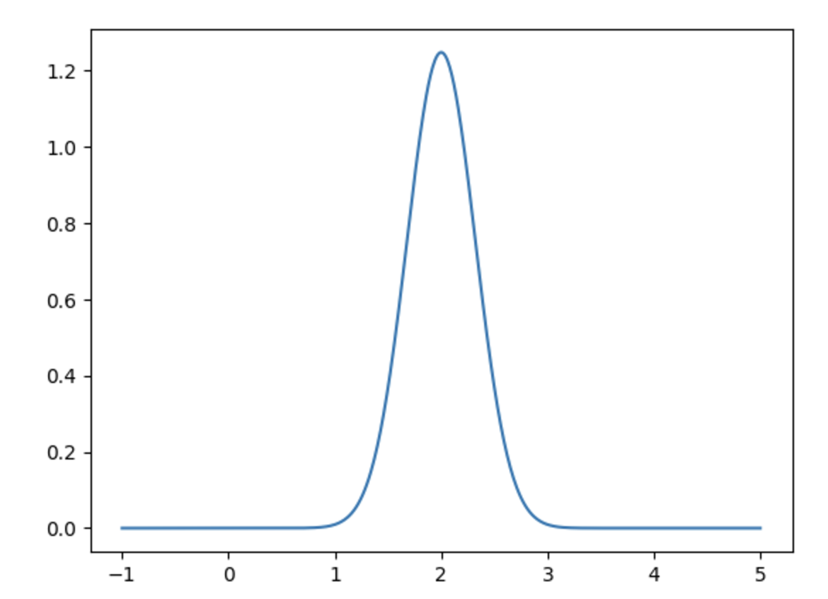
Now we at least have a reasonably intuitive interpretation of convolution in discrete probability. Our goal is to get to the integral however, so let’s see if the same idea works for probability densities. That is, we need to explore whether we get something which computes the probability density or distribution for a sum of random variables $\chi_1$ and $\chi_2$ . We can try to make this work by analogy (which is how most mathematics is done). Suppose we have functions $p_1$ and $p_2$ , where

$F_i (y) = \mathbb{P}(\{x: \chi_i (x) \leq y \}) = \int_0^y p_i (x) dx, \quad i=1,2/$

(We’re assuming the usual Lebesgue measure here, but the same will hold for your other fancy measures – hopefully. I’m assuming the $\chi_i$ are random variables over the reals with reader’s choice of appropriate $\sigma$ -algebra.) We set

$p_1 * p_2 (x) = \int p_1 (y) p_2 (x-y) dx$

and try to see if there is an analogous interpretation to the discrete case. To get some results we can make sense of without too much effort, we pick two Gaussian distributions, different enough that they are easily distinguished. This would need to be reflected in the convolution product. Let our two probability density functions be given by

$p_i (x) = \frac{1}{\sigma_i\sqrt{2\pi} } e^{-\frac{(x-\mu_i)^2}{2\sigma_i^2}}.$

Setting $\mu_1 = 0, \sigma_1 = 0.2$ and $\mu_2 = 2, \sigma_2 = 0.25$ , we get the following graphs for the density functions:

To get the convolution of the density functions $p_1$ and $p_2$ , we need to evaluate

$p_1 * p_2 (x) = \int_{-\infty}^{\infty} p_1 (x-y) p_2 (y) dy,$

which gives us the rather nasty-looking

$\frac{1}{2\pi \sigma^2 }\int_{-\infty}^{\infty} e^{-\frac{(x-y)^2}{0.08}} e^{-\frac{(y-2)^2}{0.125}} dy.$

We could try to calculate this, but instead I’m going to be lazy and just see what it looks like, which is the real point. The Python code below won’t win any prizes, and I’m not using all the library functions I could, but I think it’s pretty clear. The only (perhaps) non-obvious bit is that you have to flip an array before applying the trapezoidal method, because it’s the wrong way round, and you’ll get a negative answer otherwise:

import matplotlib.pyplot as plt
import numpy as np

def normal_dist(x, mu, sd):
    prob_density = np.exp(-0.5*((x-mu)/sd)**2)/(np.sqrt(2*np.pi)*sd)
    return prob_density

xspace = np.linspace(-1,5,601)
yspace = np.linspace(0,3,301)
valspace = []
for t in xspace:
    xyspace = t - yspace
    vals0 = normal_dist(xyspace,0.0,0.2)
    vals1 = normal_dist(yspace,2.0,0.25)
    vals2 = np.multiply(vals0,vals1)
    yspace1 = np.flip(yspace)
    valspace.append(np.trapz(yspace1,vals2))

plt.plot(xspace,valspace)
plt.show

We get the output

Compare this with the two graphs above, and test if the idea of the convolution representing the density of the sum of random variables is still valid. (Not even mentioning that the variables have to be independent, so just be aware of that.)

All of this is excellent, but what does it have to do with Fourier analysis? We’ll get to that next.

Trying to be a mathematician

Mathematics, optimisation and such

Tag Archives for convolution

What’s up with convolution (the second part)?

Interlude: What’s up with convolution? (Part the first)