You can’t even begin to do Fourier analysis without knowing about the convolution product. But this is a difficult thing to grasp intuitively. I know that I spent many hours trying to understand what’s really going on. There are, as always, really good videos on YouTube about this, which probably explain it better than I ever could, and I urge you to check them out. As for me, when I want to understand something I have to ask why this thing originated, and what it was initially used for. Something like the convolution product does not just drop out of the sky – it had to have some very definite and concrete purpose.
Fortunately, there’s a nice entry at https://math.stackexchange.com/questions/1348361/history-of-convolution that pointed me in the right way – specifically to Laplace, and the theory of probability. Let’s say you have two dice, with sides numbered from 1 to 6 as usual. What is the probability of rolling a seven? To count this we take, say, 1 and asked what should be added to make 7, which is of course 6. We do this for every other number from 2 to 6 (not taking symmetry in to account), and we add the products of the individual probabilities. In other words,

(In order to have this work for any number between 2 and 12, we would need to assign zero probability to negative numbers.). This at least looks like a convolution, and we can see if a generalization works. See if the same thing works if the second die is now 22-sided, with probabilities given by 

Now we at least have a reasonably intuitive interpretation of convolution in discrete probability. Our goal is to get to the integral however, so let’s see if the same idea works for probability densities. That is, we need to explore whether we get something which computes the probability density or distribution for a sum of random variables 


(We’re assuming the usual Lebesgue measure here, but the same will hold for your other fancy measures – hopefully. I’m assuming the 


and try to see if there is an analogous interpretation to the discrete case. To get some results we can make sense of without too much effort, we pick two Gaussian distributions, different enough that they are easily distinguished. This would need to be reflected in the convolution product. Let our two probability density functions be given by

Setting 


To get the convolution of the density functions

which gives us the rather nasty-looking

We could try to calculate this, but instead I’m going to be lazy and just see what it looks like, which is the real point. The Python code below won’t win any prizes, and I’m not using all the library functions I could, but I think it’s pretty clear. The only (perhaps) non-obvious bit is that you have to flip an array before applying the trapezoidal method, because it’s the wrong way round, and you’ll get a negative answer otherwise:
import matplotlib.pyplot as plt
import numpy as np

def normal_dist(x, mu, sd):
    prob_density = np.exp(-0.5*((x-mu)/sd)**2)/(np.sqrt(2*np.pi)*sd)
    return prob_density

xspace = np.linspace(-1,5,601)
yspace = np.linspace(0,3,301)
valspace = []
for t in xspace:
    xyspace = t - yspace
    vals0 = normal_dist(xyspace,0.0,0.2)
    vals1 = normal_dist(yspace,2.0,0.25)
    vals2 = np.multiply(vals0,vals1)
    yspace1 = np.flip(yspace)
    valspace.append(np.trapz(yspace1,vals2))

plt.plot(xspace,valspace)
plt.show
We get the output
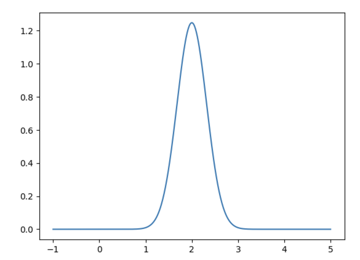
Compare this with the two graphs above, and test if the idea of the convolution representing the density of the sum of random variables is still valid. (Not even mentioning that the variables have to be independent, so just be aware of that.)
All of this is excellent, but what does it have to do with Fourier analysis? We’ll get to that next.

